Principle: Multiplying Functions (Python)
This example illustrates a central concept in Caesar.jl (and the multimodal-iSAM algorithm), whereby different probability belief functions are multiplied together. The true product between various likelihood beliefs is very complicated to compute, but a good approximations exist. In addition, ZmqCaesar offers a ZMQ interface to the factor graph solution for multilanguage support. This example is a small subset that shows how to use the ZMQ infrastructure, but avoids the larger factor graph related calls.
Products of Infinite Objects (Functionals)
Consider multiplying multiple belief density functions together, for example
\[f = f_1 \times f_2 \times f_3\]
which is a core operation required for solving the Chapman-Kolmogorov transit equations.
Direct Julia Calculation
The ApproxManifoldProducts.jl package (experimental) is meant to unify many on-manifold product operations, and can be called directly in Julia:
using ApproxManifoldProducts

f1 = manikde!(ContinuousScalar, [randn()-3.0 for _ in 1:100])
f2 = manikde!(ContinuousScalar, [randn()+3.0 for _ in 1:100])
...

f12 = manifoldProduct(ContinuousScalar, [f1;f2])
Also see previous KernelDensityEstimate.jl.
To make Caesar.jl usable from other languages, a ZMQ server interface model has been developed which can also be used to test this principle functional product operation.
Not Susceptible to Particle Depletion
The product process of say f1*f2 is not a importance sampling procedure that is commonly used in particle filtering, but instead a more advanced Bayesian inference process based on a wide variety of academic literature. The KernelDensityEstimate method is a stochastic method, what active research is looking into deterministic homotopy/continuation methods.
The easy example that demonstrates that particle depletion is avoided here, is where f1 and f2 are represented by well separated and evenly weighted samples – the Bayesian inference 'product' technique efficiently produces new (evenly weighted) samples for f12 somewhere in between f1 and f2, but clearly not overlapping the original population of samples used for f1 and f2. In contrast, conventional particle filtering measurement updates would have "de-weighted" particles of either input function and then be rejected during an eventual resampling step, thereby depleting the sample population.
Starting the ZMQ server
Caesar.jl provides a startup script for a default ZMQ instance. Start a server and allow precompilations to finish, as indicated by a printout message "waiting to receive...". More details here.
Functional Products via Python
Clone the Python GraffSDK.py code here and look at the product.py file.
import sys
sys.path.append('..')

import numpy as np
from graff.Endpoint import Endpoint
from graff.Distribution.Normal import Normal
from graff.Distribution.SampleWeights import SampleWeights
from graff.Distribution.BallTreeDensity import BallTreeDensity

from graff.Core import MultiplyDistributions

import matplotlib.pyplot as plt

if __name__ == '__main__':
    e = Endpoint()

    e.Connect('tcp://192.168.0.102:5555')
    print(e.Status())

    N = 1000
    u1 = 0.0
    s1 = 10.0
    x1 = u1+s1*np.random.randn(N)

    u2 = 50.0
    s2 = 10.0
    x2 = u2+s2*np.random.randn(N)
    b1 = BallTreeDensity('Gaussian', np.ones(N), np.ones(N), x1)
    b2 = BallTreeDensity('Gaussian', np.ones(N), np.ones(N), x2)

    rep = MultiplyDistributions(e, [b1,b2])
    print(rep)
    x = np.array(rep['points'] )
    # plt.stem(x, np.ones(len(x)) )
    plt.hist(x, bins = int(len(x)/10.0), color= 'm')
    plt.hist(x1, bins = int(len(x)/10.0),color='r')
    plt.hist(x2, bins = int(len(x)/10.0),color='b')
    plt.show()

    e.Disconnect()
A Basic Factor Graph Product Illustration
Using the factor graph methodology, we can repeat the example by adding variable and two prior factors. This can be done directly in Julia (or via ZMQ in the further Python example below)
Products of Functions (Factor Graphs in Julia)
Directly in Julia:
using IncrementalInference
fg = initfg()
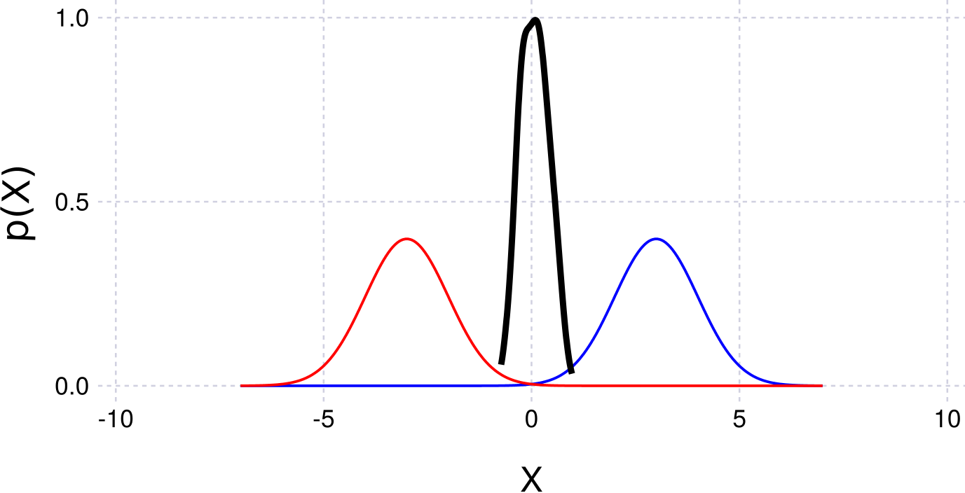
addVariable!(fg, :x0, ContinuousScalar)
addFactor!(fg, [:x0], Prior(Normal(-3.0,1.0)))
addFactor!(fg, [:x0], Prior(Normal(+3.0,1.0)))
solveTree!(fg)
# plot the results
using KernelDensityEstimatePlotting
plotKDE(getBelief(fg, :x0))Example figure:
Products of Functions (Via Python and ZmqCaesar)
We repeat the example using Python and the ZMQ interface:
import sys
sys.path.append('..')

import numpy as np
from graff.Endpoint import Endpoint
from graff.Distribution.Normal import Normal
from graff.Distribution.SampleWeights import SampleWeights
from graff.Distribution.BallTreeDensity import BallTreeDensity

from graff.Core import MultiplyDistributions


if __name__ == '__main__':
    """

    """
    e.Connect('tcp://127.0.0.1:5555')
    print(e.Status())

    # Add the first pose x0
    x0 = Variable('x0', 'ContinuousScalar')
    e.AddVariable(x0)

    # Add at a fixed location PriorPose2 to pin x0 to a starting location
    prior = Factor('Prior', ['x0'], Normal(np.zeros(1,1)-3.0, np.eye(1)) )
    e.AddFactor(prior)
    prior = Factor('Prior', ['x0'], Normal(np.zeros(1,1)+3.0, np.eye(1)) )
    e.AddFactor(prior)