Principle: Approximate Convolutions

This example illustrates a central concept of approximating the convolution of belief density functions. Convolutions are required to compute (estimate) the probabilistic chain rule with conditional probability density functions. One easy illustration is robotics where an odometry chain of poses has a continuous increase–-or spreading–-of the confidence/uncertainty of a next pose. This tutorial will demonstrate that process.

This page describes a Julia language interface, followed by a CaesarZMQ interface; a link to the mathematical description is provided thereafter.

Convolutions of Infinite Objects (Functionals)

Consider the following vehicle odometry prediction (probabilistic) operation, where odometry measurement Z is an independent stochastic process from prior belief on pose X0

\[p(X_1 | X_0, Z) \propto p(Z | X_0, X_1) p(X_0),\]

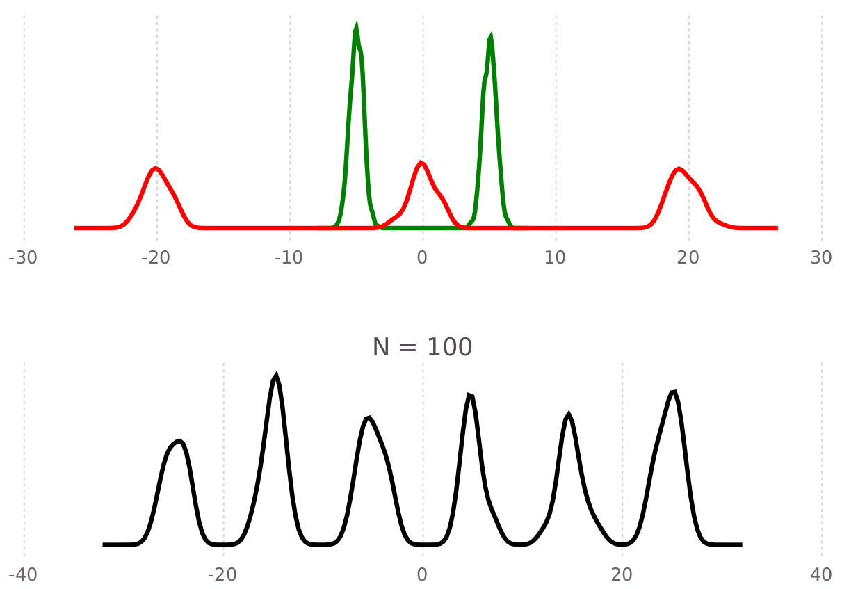
and recognize this process as a convolution operation where the prior belief on X0 is spread to a less certain prediction of pose X1. The figure below shows an example quasi-deterministic convolution of green densitty with the red density, which results in the black density below:

Note that this operation is precisely the same as a prediction step in filtering applications, where the state transition model–-usually annotated as d/dt x = f(x, z)–-is here presented by the conditional belief p(Z | X_0, X_1).

The convolution computation described above is a core operation required for solving the Chapman-Kolmogorov transit equations.

Underlying Mathematical Operations

In order to compute generic convolutions, the mmisam algorithm uses non-linear gradient descent to resolve estimates of the target variable based on the values of other dependent variables. The conditional likelihood (multidimensional factor) is based on a residual function:

\[z_i = \delta_i (\theta_i)\]

where z_i is the innovation of any smooth twice differentiable residual function delta. The residual function depends on specific variables collected as theta_i. The IIF code supports both root finding or minimization trust-region operations, which are each provided by NLsolve.jl or Optim.jl packages respectively.

The choice between root finding or minimization is a performance consideration only. Minimization of the residual squared will always work but certain situations allow direct root finding to be used. If the residual function is guaranteed to cross zero–-i.e. z*=0–-the root finding approach can be used. Each measurement function has a certain number of dimensions – e.g. ranges or bearings are dimension one, and an inter Pose2 rigid transform (delta x, y, theta) is dimension 3. If the variable being resolved has larger dimension than the measurement residual, then the minimization approach must be used.

The method of solving the target variable is to fix all other variable values and resolve, sample by sample, the particle estimates of the target. The Julia programming language has good support for functional programming and is used extensively in the IIF implementation to utilize user defined functions to resolve any variable, including the null-hypothesis and multi-hypothesis generalizations.

The following section illustrates a single convolution operation by using a few high level and some low level function calls. An additional tutorial exists where a related example in one dimension is performed as a complete factor graph solution/estimation problem.

Previous Text (to be merged here)

Proposal distributions are computed by means of (analytical or numerical – i.e. "algebraic") factor which defines a residual function:

\[\delta : S \times \Eta \rightarrow \mathcal{R}\]

where $S \times \Eta$ is the domain such that $\theta_i \in S, \, \eta \sim P(\Eta)$, and $P(\cdot)$ is a probability.

A trust-region, nonlinear gradient decent method is used to enforce the residual function $\delta (\theta_S)$ in a leave-one-out-Gibbs strategy for all the factors and variables in each clique. Each time a factor residual is enforced for another particle along with a sample from the stochastic noise term. Solutions are found either through root finding on "full dimension" equations (source code here):

\[\text{solve}_{\theta_i} ~ s.t. \, 0 = \delta(\theta_{S}; \eta)\]

Or minimization of "low dimension" equations (source code here) that might not have any roots in $\theta_i$:

\[\text{argmin}_{\theta_i} ~ [\delta(\theta_{S}; \eta)]^2\]

Gradient decent methods are obtained from the Julia Package community, namely NLsolve.jl and Optim.jl.

The factor noise term can be any samplable belief (a.k.a. IIF.SamplableBelief), either through algebraic modeling, or (critically) directly from the sensor measurement that is driven by the underlying physics process. Parametric factors (Distributions.jl) or direct physical measurement noise can be used via AliasingScalarSampler or KernelDensityEstimate.

Illustrated Calculation in Julia

The IncrementalInference.jl package provides a generic interface for estimating the convolution of full functional objects given some user specified residual or cost function. The residual/cost function is then used, with the help of non-linear gradient decent, to project/resolve a set of particles for any one variable associated with a any factor. In the binary variable factor case, such as the odometry tutorial, either pose X2 will be resolved from X1 using the user supplied likelihood residual function, or visa versa for X1 from X2.

The IncrementalInference (IIF) package provides a few generic conditional likelihood functions such as LinearRelative or MixtureRelative which we will use in this illustration.

Consider a robot traveling in one dimension, progressing along the x-axis at varying speed. Lets assume pose locations are determined by a constant delta-time rule of say one pose every second, named X0, X1, X2, and so on.

Lets a few basic factor graph operations to develop the desired convolutions:

using IncrementalInference

# empty factor graph container
fg = initfg()

# add two variables of interest
addVariable!(fg, :x0, ContinuousScalar)
addVariable!(fg, :x1, ContinuousScalar)

# gauge the solution by adding the first prior information that represents all history up to the current starting position for the robot
pr = Prior(Normal(0.0, 0.1))
addFactor!(fg, [:x0], pr)

# numerically initialize variable :x0 -- this avoids repeat computations later (specific to this tutorial)
doautoinit!(fg, :x0)

# lastly add the odometry conditional likelihood function between the two variables of interest
odo = LinearConditional(Rayleigh(...))
addFactor!(fg, [:x0;:x1], odo)  # note the list is order sensitive

The code block above (not solved yet) describes a algebraic setup exactly equivalent to the convolution equation presented at the top of this page.

To perform an stochastic approximate convolution with the odometry conditional, one can simply call a low level function used the mmisam solver:

pts = approxConvBelief(fg, :x0x1f1, :x1) |> getPoints

The approxConvBelief function call reads as a operation on fg which won't influence any values of parameter list (common Julia exclamation mark convention) and must use the first factor :x0x1f1 to resolve a convolution on target variable :x1. Implicitly, this result is based on the current estimate contained in :x0. The value of pts is a ::Array{Float64,2} where the rows represent the different dimensions (1-D in this case) and the columns are each of the different samples drawn from the intermediate posterior (i.e. convolution result).

approxConvBelief(dfg, from, target; ...)
approxConvBelief(
    dfg,
    from,
    target,
    measurement;
    solveKey,
    N,
    tfg,
    setPPEmethod,
    setPPE,
    path,
    skipSolve,
    nullSurplus
)

IIF currently uses kernel density estimation to convert discrete samples into a smooth function estimate. The sample set can be converted into an on-manifold functional object as follows:

# create kde object by referencing back the existing memory location pts
hatX1 = manikde!(ContinuousScalar, pts)

The functional object X1 is now ready for other operations such as function evaluation or product computations discussed on another principles page. The ContinuousScalar manifold is just Manifolds.TranslationGroup(1).

approxDeconv

Analogous to a 'forward' convolution calculation, we can similarly approximate the inverse:

approxDeconv(fcto; ...)
approxDeconv(fcto, ccw; N, measurement, retries)

approxDeconv(dfg, fctsym; ...)
approxDeconv(dfg, fctsym, solveKey; retries)

This feature is not yet as feature rich as the approxConvBelief function, and also requires further work to improve the consistency of the calculation – but none the less exists and is useful in many applications.